Why one label for the whole image is not enough

Classification is short. An image goes through a convolutional network and one class comes out:

[ image ]
    ↓
   CNN
    ↓
  valve

The only question is “what is depicted?”. That is honest when the frame holds one object and you do not need coordinates. A handwritten digit in an already cropped cell is that case: image → class 7.

A real frame asks three questions at once: what was found, where it is, and how sure the model is. A detector’s answer is a record, not a string:

{
  "class": "valve",
  "confidence": 0.96,
  "bbox": [120, 240, 180, 310]
}

bbox is the bounding box: a rectangle around the object. The numbers are pixels of the corners, or the equivalent “center, width, height.” The point is the same: the object is tied to a place on the sheet.

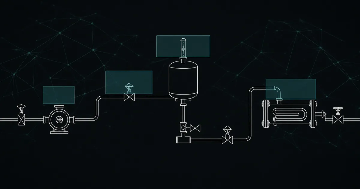
A process diagram in one frame holds a pump, valves, a heat exchanger, a tank, instruments, and text tags. A single classifier on the whole sheet is forced to pick a “main” class and drop the rest. You can slice the sheet into hundreds of crops and classify each, but then you have invented a detector — slower, and without a shared picture. Detection exists so you do not have to do that by hand.

What YOLO is, and what it is not

YOLO stands for You Only Look Once. The idea: the image passes through the model, and the model emits a set of detected objects instead of searching with a sliding window.

                 IMAGE
                   ↓
               YOLO model
                   ↓
     ┌─────────────┼─────────────┐
     ↓             ↓             ↓
   pump          valve          tank

Do not collapse four different things into “the YOLO model”:

• the idea and the family — one pass, boxes and classes;
• a specific version — early grids and modern heads are not the same machine;
• a weight file — the numbers the network has learned;
• a pretrained model — weights trained on a general set such as everyday photos;
• your model — those starting weights after fine-tuning on your diagrams.

Early versions did split the picture into a fixed grid and predict a few boxes per cell. Current implementations moved on: anchors, anchor-free heads, separate heads at several scales. For an engineer the output contract matters — class, box, confidence — not the 2016 grid story.

The family stays popular because of a combination, not magic. Inference is fast. Quality on a narrow task is reachable by fine-tuning. Box labels are cheaper than full masks. Pretrained weights transfer visual features. Some builds also cover segmentation and keypoints. For a first industrial detector that is more practical than designing an architecture from scratch.

Three problem statements: class, box, and mask

The comparison is short, and the labeling budget depends on it.

Classification: image → class. One label, no place.

Detection: image → class + bbox + confidence. Several objects, each with a rectangle and a score.

Segmentation: image → class + pixel mask. The class is assigned to pixels, not to a rectangle. The mask follows the shape.

For equipment a box is usually enough. A pump, a valve, a tank are compact symbols:

┌────────────┐
│   P-101    │
└────────────┘

For a pipeline a box is crude. A pipe can turn across half the sheet, and the rectangle swallows empty space and foreign symbols:

┌─────────────────────────────┐
│                             │
└─────────────────────────────┘

Segmentation marks the line itself. It costs more to label and to train, and the connection geometry stops being a guess from rectangle corners. The same fork shows up on a weld: a box fits a compact defect, a mask is for area and shape. On a diagram the rule is the same. Equipment gets boxes. Process lines get masks if “what connects to what” is part of the product contract.

How the network sees a frame

A detector is a convolutional network with a head that turns features into boxes. Early layers notice edges, lines, corners, and simple shapes. Deeper layers assemble parts and characteristic silhouettes: a valve circle, a pump body, a tank outline. That is not “understanding a P&ID standard.” It is the statistics of shapes the network learned from your labels.

Three roles inside a modern YOLO are enough.

The backbone extracts features. Pretrained weights help here: edges and textures are already something almost any photo-trained network can see.

The neck mixes features at several scales. A small instrument and a large tank do not live at one resolution of the feature map. Without multi-scale features a small symbol on a large sheet disappears — the same failure as a weld-defect detector without tiling.

The detection head turns feature maps into predictions: coordinates, class, confidence. This is what fine-tuning moves most when the domain is new and the backbone already “sees.”

What the detector actually predicts

A box is four numbers. Often center, width, and height; sometimes corners. In a YOLO label file they are normalized: divided by image width and height, so they lie between 0 and 1. The same label survives a resize.

The class is an integer from your vocabulary:

0 = pump
1 = valve
2 = tank
3 = exchanger

The network does not “know the word pump.” It emits a distribution over indices. The class name lives in a config next to the weights. Reorder the vocabulary and skip retraining, and you have silently renamed a pump into a valve.

Confidence is the score attached to a box. You use it as a threshold: drop below 0.25, keep the rest. It is not a calibrated probability. 0.96 does not mean “a valve is here in 96 of 100 cases” until you check calibration on your own test. The threshold is a lever between precision and recall, not a physical fact.

The same class can appear many times on one sheet:

pump
pump
pump
valve
valve

A detector is built for that list. A whole-image classifier will not return it.

How one model finds many objects

A single pass means the network is not restarted on every possible rectangle. It looks at feature maps and proposes many candidates, at several scales and places. Most candidates are background. A confidence threshold cuts them.

Then a practical nuisance remains: for one valve the model often proposes several overlapping boxes.

        ┌───────────────┐
        │     valve     │
        └───────────────┘

   ┌──────────────┐
   │    valve     │
   └──────────────┘

Non-maximum suppression (NMS) keeps the box with the highest confidence and drops neighbors that overlap it too much. Overlap is measured by intersection.

Intersection over union (IoU):

IoU = intersection area / union area

Nearly identical boxes give an IoU close to 1. Boxes that barely touch sit near 0. The NMS threshold says when two predictions are duplicates of one object. A separate confidence threshold says which candidates reach that step at all.

IoU is not only post-processing. Evaluation uses it to decide whether a predicted box matches ground truth. The class can be right while the box has slid onto the next symbol — that is not a hit if the overlap is below the agreed threshold. A bare “mAP 0.8” is not a report: name the method and the IoU thresholds.

Your own model: pretrained weights and fine-tuning

You do not assemble a custom YOLO from random layers on day one. The usual path is:

pretrained YOLO weights
       ↓
your dataset
       ↓
fine-tuning
       ↓
your diagram detector

Pretrained weights are a network that already extracts edges, corners, and coarse object shapes from ordinary photos. It has not seen your drawing standard. It has seen enough of the visual world that you do not have to teach “what a line is” from scratch.

Transfer learning adapts those skills to a new domain. Someone who already reads another plant’s drawings learns your symbols faster than someone seeing a line on paper for the first time. Backbone weights are that existing skill. Fine-tuning moves them toward your symbols.

Training from scratch looks different:

random weights
      ↓
a large set
      ↓
a long training run

It is justified when the domain is visually far from photographs, the set is huge, and pretrained weights keep getting in the way. For a first detector of pumps and valves it is almost always the worse start: slower, costlier, easier to fail to converge. Fine-tuning is not a quality guarantee. It is a sane starting point. Bad labels will ruin it anyway.

When fine-tuning is the right tool, and when the data should be fixed first, is in when fine-tuning is needed. Dataset discipline, not the checkpoint, is in dataset engineering.

The dataset: labels, splits, and errors as new examples

A YOLO set is pairs of files:

images/
labels/

An image scheme-014.jpg and a label scheme-014.txt with the same stem. Each line is one object:

0 0.52 0.41 0.10 0.14

The first number is the class index. Then center x, center y, width, and height, all between 0 and 1 relative to the frame. 0.52 0.41 is slightly right of and above the middle. 0.10 0.14 occupies about a tenth of the width and a seventh of the height. A wrong class index is invisible on the box: the rectangle is right, the name is wrong. Those errors quietly damage precision.

Split the set in three. Train moves the weights. Validation shows whether the network memorized the training sheets, and you pick thresholds and the stopping point on it. Test is touched rarely: an independent score before you talk about quality, not another knob. The most common leak on diagrams is putting near-duplicate versions of one sheet into both train and validation. The network “recognizes the sheet,” the metric lies, and a new drawing standard falls apart. Split by document and by source, not by random files from one folder.

There is no universal “you need exactly 1000 images.” What matters is diversity, the number of objects (one sheet can hold dozens), difficulty, box quality, and whether inputs look like the future stream: scan, photo, CAD export, another contrast. Class balance breaks rare symbols:

pump       5000
valve       800
tank        150

The network will honestly learn the pump and miss the tank. A bigger model does not fix that. More examples of the rare class do, plus a per-class metric instead of one average.

Model errors are the next data source. The loop is shorter than any architecture argument:

set → training → model → errors → hard examples → set+ → train again

A hard example is a frame the current model already missed: glare, a nonstandard symbol, a dense valve cluster, a foreign title block. You label it and put it back. The same habit as in a form pilot: a disputed field is not “fixed by a slogan,” it goes into the reference set.

Augmentation is synthetic distortion during training: scale, crop, rotation, brightness, noise, blur, perspective, compression traces. It helps when it imitates the real input. On diagrams it is dangerous when it changes meaning: a flip can reverse flow direction, a hard rotation can turn a legal symbol into an illegal one. Distort only what you are willing to see in production.

How training runs, and whether you need a GPU

The loop is the same as for any trained network, except the loss looks at three things at once: whether an object is there, where the box is, and which class it is.

image → forward pass → prediction → loss → backpropagation → weight update

Loss details depend on the family version. You do not need to memorize them in a first article. The contract is enough: the network is penalized for a miss, for a shifted box, and for a wrong class. You cannot “classify well” while stably drawing the box on the neighboring symbol — the combined loss will punish that.

An epoch is one pass over the training set. A batch is the pack of images used for one update. The learning rate is the step size. Too large a step scatters the weights; too small a step stalls. Overfitting shows up as a pair of curves: training quality rises, validation quality falls. The network memorized sheets, not symbols.

A GPU is worth having for training: the same fine-tune takes minutes or hours instead of a day. Inference is different. One sheet a second often fits on a CPU. A GPU at inference is for a large stream, a hard latency budget, or a heavy model. Training and production are different machines:

training machine
     ↓
weights / ONNX
     ↓
CPU inference server

A GPU in the experiment does not imply a GPU next to the customer’s service.

How to measure quality, and which errors to count

Precision: of everything the model found, what fraction was right. Low precision means many false alarms.

Recall: of everything that was on the sheet, what fraction the model found. Low recall means misses.

A cautious model rarely lies and often misses. An aggressive model finds almost everything and clutters the frame. The confidence threshold moves you along that axis. On a diagram a missed valve and a false valve cost different money; pick the threshold by the cost of the error, not by a pretty average.

AP (average precision) compresses the precision-recall curve of one class into one number. mAP is the mean of AP across classes. It depends on IoU thresholds and on how a hit is defined. Compare two models only under the same method. One class with five examples can wreck or paint the average — read the per-class table.

Typical errors are more useful than one figure:

• false positive — a valve where there is none;
• false negative — a valve is there, no box;
• classification error — a pump named as a heat exchanger, box in the right place;
• localization error — right class, shifted box;
• duplicate — one object, two boxes, NMS did not suppress them.

Misses hide easily if you only watch precision. On a diagram a miss is often more expensive than an extra box: the absent valve never enters the graph.

What beats architecture

The order of influence on a first release is almost always:

1. image quality;
2. box and class-index quality;
3. diversity of sources;
4. an honest train / validation / test split;
5. putting hard errors back into the set;
6. learning rate, epochs, thresholds;
7. architecture size and name.

A larger model does not compensate for a bad set. It costs more to train, memorizes bad labels more eagerly, and runs slower at inference. Start with a small or mid-size head on clean boxes. Grow the architecture when the ceiling is measured, not when “that is what this year does.”

YOLO on process diagrams

On a P&ID and similar drawings, give the detector compact symbols: pump, valve, tank, compressor, heat exchanger, filter, sensor, instrument, motor. The vocabulary should be one you can label consistently. A hundred classes “just in case” dilute rare symbols and break name agreement.

Text is a separate decision.

Approach A: the detector finds text regions, and the crop goes to recognition (OCR / CRNN). The plus is that text is tied to a box, so matching it to a nearby symbol is easier. The minus is another class to label, and dependence on how the detector cuts the line.

Approach B: a separate system finds and reads text on its own. The plus is that you do not mix equipment and character vocabularies. The minus is that matching “tag P-101 belongs to this pump” becomes a geometry problem after both pipelines.

On forms we already saw a general vision model on the whole sheet confuse empty cells and geometry. The lesson on a diagram is the same: a symbol detector should not also be the only reader of tags. The task split is:

YOLO → where is the object?
CRNN / OCR → what is written?
Segmentation → where does the line run?
Graph builder → what connects to what?
Language model → what does that structure mean?

Specialized models are not competing here. They answer different questions. A CRNN is strong on a character sequence and weak as a pump finder. YOLO is strong as a pump finder and does not read P-101. Modern OCR is not always a CRNN — the contract “a string on a crop” matters, not the architecture name.

Why a detector does not understand a diagram

After a good run you have a list:

P-101 — pump
V-101 — valve
E-101 — exchanger

That is not enough to claim:

P-101 → V-101 → E-101

Boxes do not store flow direction, and they do not know which line is which when pipes cross. Detection is not understanding. Understanding starts when objects, tags, and lines are assembled into a graph, and the graph is checked by rules: a valve with no line, a tag hanging in empty space, a tag that disagrees with the symbol type.

A language model can be attached in two ways.

The first is to hand it the picture and ask for an answer. Fast prototype, convenient exploration. Weak spots: completeness over the whole sheet is hard to guarantee, coordinates drift, connections on a large drawing get lost, and the same sheet is not obliged to yield the same graph twice.

The second is vision and geometry first, then structure, then the model:

image → vision → structure → language model

That is easier to validate, easier to apply engineering rules to, and harder to confuse with “the model told a fluent story” when not every valve was found. Here the language model interprets the graph: analogies, an explanation of the loop, answers against a knowledge base. It does not draw the missing box.

A pipeline of several models

Draw this frame before you pick weights:

                   SCHEME
                      │
                      ▼
                preprocessing
                      │
         ┌────────────┴────────────┐
         ▼                         ▼
    symbol detection             text
         │                         │
         ▼                         ▼
     equipment                 string reading
         │                         │
         └────────────┬────────────┘
                      ▼
               lines and geometry
                      │
                      ▼
                connection logic
                      │
                      ▼
                     GRAPH
                      │
                      ▼
           rules and a language model

Preprocessing is scan rotation, margin crop, a shared scale. Without it the detector learns crooked photos instead of symbols. Then two parallel vision paths: symbols and text. Then lines. Then connection rules: which object touches which line, which tag is closest to which symbol (P-101 → pump, V-101 → valve). The graph is the first product you can test without a conversation about “intelligence.” The language model and knowledge search sit above it.

A roadmap by stages, not one release:

1. Equipment detector
2. Tag reading
3. Lines
4. Connection geometry
5. Graph
6. Engineering checks
7. Interpretation and knowledge search

Each stage has its own test. You cannot close stage 1 with the metric of stage 7.

A small project, inference, and production

A short teaching detector is assembled like this. One to three hundred images. Three to five classes: pump, valve, tank if you have drawings, or everyday objects if you do not yet. Boxes. A split without near-duplicate leaks. Pretrained weights. Fine-tuning. Precision, recall, mAP, and a mandatory look at errors. Hard frames back into the set. Repeat.

That is a protocol, not a run report. Plan several passes and do not watch a single number: a baseline, a pass with cautious augmentation, a pass with hard examples, a pass with a larger set, and threshold tuning after the weights are frozen. Thresholds do not retrain the network — they pick an operating point of precision and recall.

After training you have weights. A training-format file is not yet production. Next is export for a specific runtime: the native format, ONNX, and if needed an accelerator such as TensorRT. Pick the format for where the model will live, not for fashion.

Inference on one frame:

image
 ↓
resize / preprocessing
 ↓
detector
 ↓
confidence filter
 ↓
duplicate suppression
 ↓
JSON

{
  "objects": [
    {
      "class": "pump",
      "confidence": 0.97,
      "bbox": [120, 200, 240, 320]
    }
  ]
}

Production is latency, throughput, memory, file size, a container, a weight version, and monitoring of errors on live sheets. “97% on the test set” describes none of those. After release the loop is the same as for the dataset: live errors → labeling → a new data version → training → evaluation → release. A model is not “finished forever” at the first weight file.

Common mistakes

Reaching for the largest model before the rare class is labeled.

Too few images, all from one exporter. On a foreign title block the detector goes blind.

Crooked boxes, swapped class indices, the same symbol labeled differently by two people.

Near-duplicate sheets in both train and validation.

Watching one mAP and never opening the misses.

Asking one YOLO to find the pump, read the tag, and rebuild the graph.

Treating fine-tuning itself as proof the model is good.

Ignoring duplicates and thresholds, then arguing about the weights.

FAQ

Further reading

Nearby on this site are pipelines this detector grows out of, rather than replaces.

• Teaching a network to read handwritten digits — class versus sequence, and when a heavy recognizer is unnecessary.
• A compact CRNN for measurements — reading a short string on a crop.
• Why one model is not enough on a form — geometry, confidence, and a human in the loop.
• Vision on a weld radiograph — box versus mask on an industrial frame.
• Dataset engineering — dataset versions, leaks, and a reference set.
• When fine-tuning is needed — fine-tuning as a behavior change, not a document warehouse.
• How language models are trained — so the detector and the interpretation layer stay distinct.

The next practical piece in this line is a walkthrough of training on P&ID: class vocabulary, a labeling tool, the training config, a confusion matrix, and export to ONNX. It is worth writing once a run has been measured, not from a plan of a run.

Conclusion

YOLO does not “understand the picture.” It learns to find objects of chosen classes and to mark where they are. On a process diagram that is enough to lift off the equipment layer, and not enough to know what connects to what or what is written beside it.

Start your own model from pretrained weights, a narrow vocabulary, and honest labels. Hold quality by recall and misses, not by one average score. A GPU speeds training and does not have to sit next to every inference server.

An intelligent pipeline appears when the detector stands next to text reading, lines, graph rules, and only then a language model. A useful minimum this week is to label fifty sheets with three classes and see which symbols the network confuses. That error list is worth more than an architecture change before the first run.